Notes about jQuery-UI (july 19)

Make sure that the jquery-ui object is loaded by using the DOM inspector.
https://learn.jquery.com/jquery-ui/environments/amd/
http://www.requirejs.org/jqueryui-amd/example/webapp/app.html
https://gist.github.com/diestrin/8509552
http://hippieitgeek.blogspot.com/2013/07/load-jquery-ui-with-requirejs.html
http://gregfranko.com/blog/registering-the-jqueryui-widget-factory-as-an-amd-module/
http://blog.dbain.com/2016/02/using-requirejs-to-load-jquery-ui-from.html
 (use the above examples)

Getting Jupyter Server started

For Jupyter Notebook use python3 (python3 --version => 3.4), (which python3 /usr/local/bin/python3)

Install Jupyter Notebook with pip (pip3 install ---upgrade pip), (pip3 install jupyter)

Start the Jupyter server in directory where you have permissions such as $home/Documents/ (jupyter notebook)

Reference (https://jupyter.readthedocs.io/en/latest/install.html)

Set up the python packages (modules)

sudo pip3 install beautifulsoup4
sudo pip3 install nltk

sudo pip3 install numpy
sudo pip3 install scipy
sudo pip3 install sklearn

Running Jupyter:

In $home/Documents: jupyter notebook

Run the script:

from bs4 import BeautifulSoup
import nltk
from nltk.corpus import stopwords
from sklearn.feature_extraction.text import TfidfVectorizer
from sklearn.decomposition import TruncatedSVD

cds = open('/home/brent/Downloads/cd_catalog.xml').read()
print(cds)
soup = BeautifulSoup(cds)
postTxt = soup.findAll('artist')
postDocs = [x.text for x in postTxt]
print(postDocs)
postDocs.pop[0]   (error postDocs is not scriptable)
postDocs = [x.lower() for x in postDocs]     (changes everything to lowercase)

stopset.update(['lt','p','/p','br','amp','quot','field','front','normal','span','Opx','rgb','style','51','spacing','text','helvetica','size','family','space','arial','height','indent','letter','line','none','sans','serif','transform','line','variant','weight','times','new','strong','video','title','white','word','letter','roman','0pt','16','color','12','14','21','neue','apple','class',
               ])
 

print(postDocs)
stopset = set(stopwords.words('english'))

Links found Looking for Latent Semantic Analysis (originally to find what Latent means)

Probabilistic Latent Semantic Analysis
http://web.mit.edu/~punk/Public/AudioExtraction/PLCApage.html

Latent Semantic Analysis
https://en.wikipedia.org/wiki/Latent_semantic_analysis

Text Analytics - Latent Semantic Analysis
https://www.youtube.com/watch?v=BJ0MnawUpaU
From Playlist:
https://www.youtube.com/watch?v=Jh1kuqm4rMc&list=PLlWzRW5RWfEX-HeTjCDWTRCOhISKrPAep

try replicating the last video with Jupyter: http://jupyter.readthedocs.io/en/latest/install.html

Links Found Looking for Linked Data and Machine Learning

"Choosing a Machine Learning Classifier" http://blog.echen.me/2011/04/27/choosing-a-machine-learning-classifier/


"3rd International Workshop on Inductive Reasoning and Machine Learning for the Semantic Web"  https://sites.google.com/site/irmles2011/


 "Volker Tresp's Homepage" http://www.dbs.ifi.lmu.de/~tresp/


Maximilian Nickel, Volker Tresp, Hans-Peter Kriegel "Factorinzing Yago" http://www.dbs.ifi.lmu.de/%7Etresp/papers/p271.pdf

(edit: see the RESCAL paper this is based on: "A Three-Way Model for Collective Learning on Multi-Relational Data"
http://www.icml-2011.org/papers/438_icmlpaper.pdf )

 Volker Tresp's student Maximilian Nickel's Homepage: http://web.mit.edu/~mnick/www/

 Maximilian Nickel's Development RESCAL: https://github.com/mnick/rescal.py

Extension EX-RESCAL: https://github.com/researchstudio-sat/webofneeds/tree/master/webofneeds/won-matcher-rescal/src/main/python/extrescal Conclusion: Factorizing Yago is useful for understanding EX-RESCAL

Notes for Logistic regression in R on July 5th

Steps to take for Logistic Regression in R:

(1) Load data
(2) attach(data-sample)
(3) summary(data-sample)
(4) ced.del <- cbind(sDel, sNoDel)
(5) summary(ced.del)
(6) duckie <- glm(ced.del ~ cat + follows + factor(class), family=binomial)
(7) duckie
(8) summary(duckie)
(9) anova(duckie, test="Chisq")
(10) plot(duckie)

Revised:

fico <- read.table("/home/brent/Documents/fico.csv", header=TRUE, sep=",",
  na.strings="NA", dec=".", strip.white=TRUE)

attach(fico)

duckie <- glm(approved ~ creditScore, family=binomial)

summary(duckie)

------

> summary(duckie)

Call:
glm(formula = approved ~ creditScore, family = binomial)

Deviance Residuals:
   Min      1Q  Median      3Q     Max 
-1.408  -1.338   0.959   1.010   1.149 

Coefficients:
             Estimate Std. Error z value Pr(>|z|)
(Intercept) -6.223592  17.177351  -0.362    0.717
creditScore  0.009605   0.024893   0.386    0.700

(Dispersion parameter for binomial family taken to be 1)

    Null deviance: 20.190  on 14  degrees of freedom
Residual deviance: 20.038  on 13  degrees of freedom
AIC: 24.038

Number of Fisher Scoring iterations: 4

Use the intercept and the credit score to solve for the predicted probability:

With the coefficient estimates we have:

Notes on July 3rd

JQuery, Python, and Deep Learning Resources:

https://www.npmjs.com/package/jquery-ui

https://peter.pudaite.net/2017/05/21/learning-tensorflow-without-a-background-in-machine-learning/

Learning Python - Fabrizio Romano 

Machine Learning Recipes with Josh Gordon -- https://goo.gl/KewA03

https://www.udemy.com/data-science-deep-learning-in-python/

Linear Regression Notes

How to Replicate Example 10.1 in Statistics... by Mendenhall et al, 5th Ed, in R:

Y <- c(1,1,2,2,4)
X <- c(1,2,3,4,5)
fit <- lm(Y ~ X)
plot(X,Y,xlim=c(0,5),ylim=c(-1,4))
abline(fit)

> lm(Y ~ X)

Call:
lm(formula = Y ~ X)

Coefficients:
(Intercept)            X 
       -0.1          0.7

> plot(X,Y,xlim=c(0,5),ylim=c(-1,4))
> abline(fit)



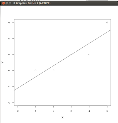
> summary(fit)

Call:
lm(formula = Y ~ X)

Residuals:
         1          2          3          4          5
 4.000e-01 -3.000e-01 -6.891e-17 -7.000e-01  6.000e-01

Coefficients:
            Estimate Std. Error t value Pr(>|t|) 
(Intercept)  -0.1000     0.6351  -0.157   0.8849 
X             0.7000     0.1915   3.656   0.0354 *
---
Signif. codes:  0 '***' 0.001 '**' 0.01 '*' 0.05 '.' 0.1 ' ' 1

Residual standard error: 0.6055 on 3 degrees of freedom
Multiple R-squared: 0.8167,    Adjusted R-squared: 0.7556
F-statistic: 13.36 on 1 and 3 DF,  p-value: 0.03535

Link used for reference:
Using R for Linear Regression<http://www.montefiore.ulg.ac.be/~kvansteen/GBIO0009-1/ac20092010/Class8/Using%20R%20for%20linear%20regression.pdf>
<http://www.statmethods.net/advgraphs/axes.html>
<http://www.dummies.com/programming/r/how-to-add-variables-to-a-data-frame-in-r/>